Sort

La Cité Paris, 1934, Paul Signac
- 1. Bubble Sort
- 2. Selection Sort
- 3. Insertion Sort
- 4. Quick Sort
- 5. Counting Sort
- 6. Radix Sort
- 7. Merge Sort
- 8. Heap Sort
- 9. Sort Algorithm Comparison
- 10. Sort Example Problem
Sorting is arranging data in order according to a specific criterion.
In general, an appropriate sorting algorithm is used as a formula according to the problem situation.
1. Bubble Sort
1.1 What is Bubble Sort?
Bubble sort is a sorting algorithm that compares two adjacent elements and swaps them until the list is sorted.
Just like the movement of air bubbles in the water that rise up to the surface, each element of the array move to the end in each iteration. Therefore, it is called a bubble sort.
[Step 0]
First Iteration (Compare and Swap)
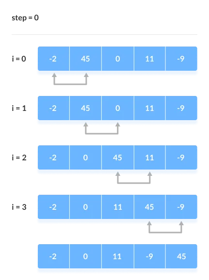
- Starting from the first index, compare the first and the second elements.
- If the first element is greater than the second element, they are swapped.
- Now, compare the second and the third elements. Swap them if they are not in order.
- The above process goes on until the last element.
[Step 1]
Remaining Iteration
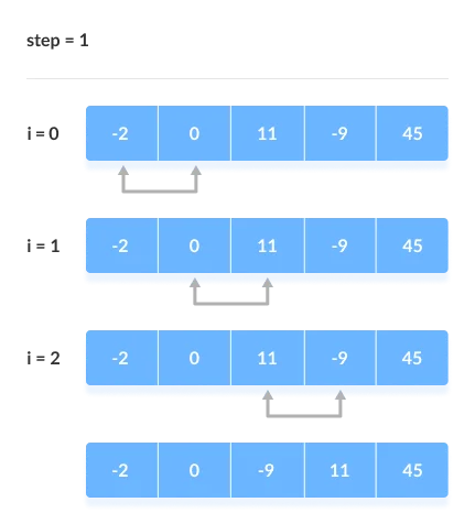
The same process goes on for the remaining iterations.
After each iteration, the largest element among the unsorted elements is placed at the end.
[Step 2]
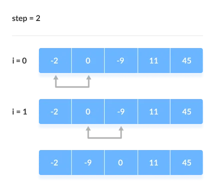
In each iteration, the comparison takes place up to the last unsorted element.
[Step 3]
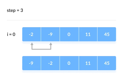
The array is sorted when all the unsorted elements are placed at their correct positions.
1.2 Bubble Sort Implementation
# title: 'BubbleSort.py'
def bubbleSort(array):

  # loop to access each array element
  for i in range(len(array)):

    # loop to compare array elements
    for j in range(0, len(array) - i - 1):

      # compare two adjacent elements
      # change > to < to sort in descending order
      if array[j] > array[j + 1]:

        # swapping elements if elements
        # are not in the intended order
        temp = array[j]
        array[j] = array[j+1]
        array[j+1] = temp


data = [-2, 45, 0, 11, -9]

bubbleSort(data)

print('Sorted Array in Ascending Order:')
print(data)
Optimized Bubble Sort Algorithm
In the above algorithm, all the comparisons are made even if the array is already sorted.
This increases the execution time.
To solve this, we can introduce an extra variable swapped. The value of swapped is set true if there occurs swapping of elements. Otherwise, it is set false.
After an iteration, if there is no swapping, the value of swapped will be false. This means elements are already sorted and there is no need to perform further iterations.
This will reduce the execution time and helps to optimize the bubble sort.
# title: 'OptimizedBubbleSort.py'
# Optimized Bubble sort in Python

def bubbleSort(array):

  # loop through each element of array
  for i in range(len(array)):

    # keep track of swapping
    swapped = False

    # loop to compare array elements
    for j in range(0, len(array) - i - 1):

      # compare two adjacent elements
      # change > to < to sort in descending order
      if array[j] > array[j + 1]:

        # swapping occurs if elements
        # are not in the intended order
        temp = array[j]
        array[j] = array[j+1]
        array[j+1] = temp

        swapped = True

    # no swapping means the array is already sorted
    # so no need for further comparison
    if not swapped:
      break

data = [-2, 45, 0, 11, -9]

bubbleSort(data)

print('Sorted Array in Ascending Order:')
print(data)
1.3 Time Complexity of Bubble Sort
Time Complexities
Worst Case Complexity: \(O(N^2)\)
- If we want to sort in ascending order and the array is in descending order then the worst case occurs.
Best Case Complexity: \(O(N)\)
- If the array is already sorted, then there is no need for sorting.
Average Case Complexity: \(\underline{O(N^2)}\)
- It occurs when the elements of the array are in jumbled order (neither ascending nor descending).
Space Complexity
Space complexity is \(O(1)\) because an extra variable is used for swapping.
In the optimized bubble sort algorithm, two extra variables are used. Hence, the space complexity will be \(O(2)\).
1.4 Bubble Sort Applications
- complexity does not matter
- short and simple code is preferred
2. Selection Sort
2.1 What is Selection Sort?
It repeats selecting the smallest data among the unprocessed data and replacing it with the first data.
[Step 0]
Select the smallest 0 among unprocessed data and replace it with the leading 7. 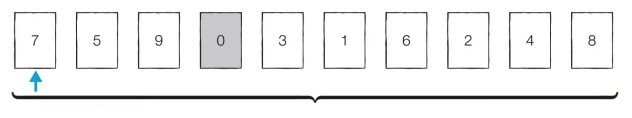
[Step 1]
Select the smallest 1 among unprocessed data and replace it with the leading 5. 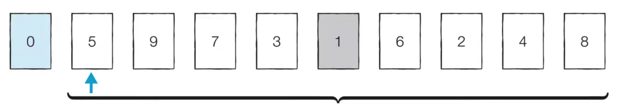
[Step 2]
Select the smallest 2 among unprocessed data and replace it with the leading 9. 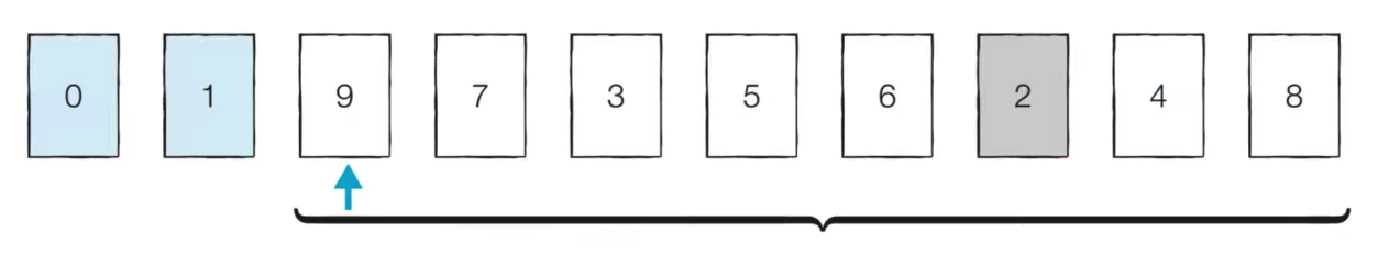
[Step 3]
Select the smallest 3 among unprocessed data and replace it with the the leading 7. 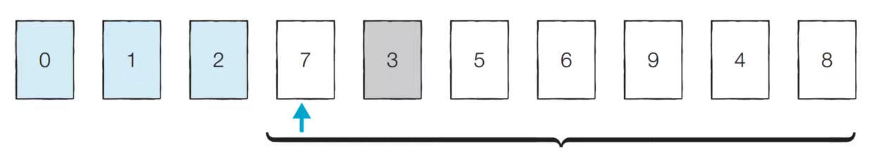
[Step 8]
If this process is repeated, the sorting is completed as follows. 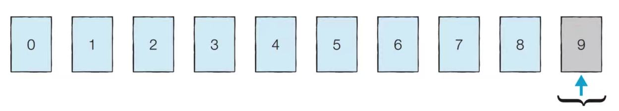
The search range decreases with each iteration. Each time, the data is checked as far as the search range to find the smallest element. It is equivalent to doing a linear search every time.
2.2 Selection Sort Implementation
# title: 'SelectionSort.py'
array = [7, 5, 9, 0, 3, 1, 6, 2, 4, 8]

for i in range(len (array) ); # i is the smallest data and the index to change position = the frontmost position each time
    min_index = i #index of the smallest element, put the smallest element first
    for j in range( i+1, len(array) ): # j starts a linear search (from the next index)
        if array[ min_index ] > array[j]: #if there is an index smaller than the current smallest element
            min_index = j # Make the position index value come to the smallest index value
    array[i], array[min_index] = array[min_index], array[i] # swap, swap the first and smallest elements

print(array)

# output
# [0, 1, 2, 3, 4, 5, 6, 7, 8, 9]
2.3 Time complexity of Selection Sort
Selection sort must find the smallest number N times and send it to the front.
There may be minor errors depending on the implementation method, but the total number of operations is as follows.
\(N + (N -1) + (N - 2) + ... + 2\) (in arithmetic sequence form)
This can be expressed as \((N^2 + N - 2) / 2\) , which is written as \(\underline{O(N^2)}\) according to Big O notation.
2.4 Selection Sort Applications
- a small list is to be sorted
- cost of swapping does not matter
- checking of all the elements is compulsory
- cost of writing to a memory matters like in flash memory (number of writes/swaps is \(O(N)\) as compared to \(O(N^2)\) of bubble sort)
3. Insertion Sort
3.1 What is Insertion Sort?
It picks out the unprocessed data one by one and inserts them in the appropriate places.
It is more difficult to implement than selection sort, but it is generally more efficient.
[Step 0]
It is judged that the first data 7 is sorted by itself, and the position of the second data 5 is determined. There are only two cases, either going to the left of 7 or going to the right.
5 is smaller, so it goes to the left. 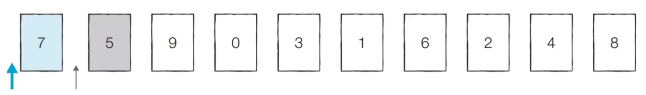
[Step 1]
Then, it is decided which position the 9 is going.
9 is bigger, so it goes right. 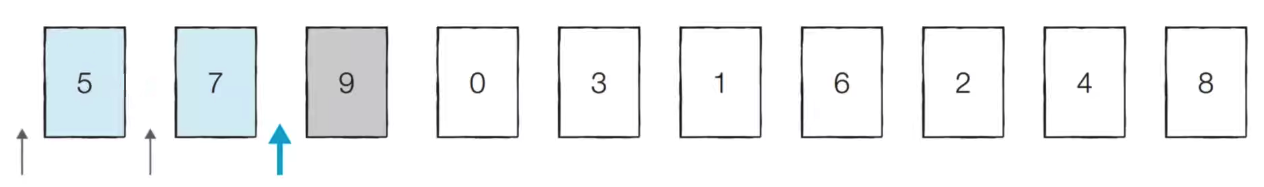
[Step 2]
Then, it is determined where the 0 is going.
Since 0 is less than 5, it is shifted to the left. 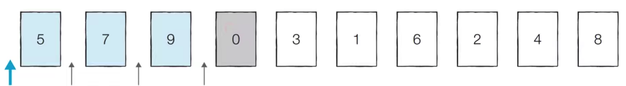
[Step 8]
If this process is repeated, the sorting is completed as follows. 
3.2 Insertion Sort Implementation
# title: 'InsertionSort.py'
array = [7, 5, 9, 0, 3, 1, 6, 2, 4, 8]

for i in range(1, len(array)): # iterate starting from the second element
    for j in range( i, 0, -1 ): # Grammar that repeats decreasing by 1 from index i to 1, where j is the position of the element to be inserted
        if array[ j ] < array[ j -1 ] #if it is less than the left
            array[ j ], array[ j -1 ] = array[ j -1 ], array[ j ] #swapping, reposition = move left
        else: #if it is greater than or equal to left
            break #stop

print(array)

# output
# [0, 1, 2, 3, 4, 5, 6, 7, 8, 9]
Receive the callback function as the second argument, and Sort the elements based on the return value of that function it is as follows.
// title: 'InsertionSort.js'
const insertionSort = function (arr, transform = (item) => item) {
  let sorted = [arr[0]];
  for (let i = 1; i < arr.length; i++) {
    if (transform(arr[i]) >= transform(sorted[i - 1])) {
      sorted.push(arr[i]);
    } else {
      for (let j = 0; j < i; j++) {
        if (transform(arr[i]) <= transform(sorted[j])) {
          const left = sorted.slice(0, j);
          const right = sorted.slice(j);
          sorted = left.concat(arr[i], right);
          break;
        }
      }
    }
  }
  return sorted;
};
3.3 Time complexity of Insertion Sort
The time complexity of insertion sort is \(\underline{O(N^2)}\), and like selection sort, the loop is used twice.
Insertion sort works very quickly if the data in the current list is almost sorted.
- It has a time complexity of \(\underline{O(N)}\) in the best case.
- What happens if you perform insertion sort again while already sorted?
-> Stops immediately while performing the search.
3.4 Insertion Sort Applications
- the array is has a small number of elements
- there are only a few elements left to be sorted
4. Quick Sort
4.1 What is Quick Sort?
This is a method of setting the reference data and changing the positions of larger and smaller data than the standard.
It is one of the most used sorting algorithms in general situations. Along with merge sort, it is an algorithm that is the basis of sort libraries in most programming languages.
The most basic quick sort sets the first data as the reference data (Pivot).
[Step 0]
The current pivot value is 5. Since data larger than 5 is selected from the left, 7 is selected, and since data smaller than 5 is selected from the right, 4 is selected. Now we swap the positions of these two data. 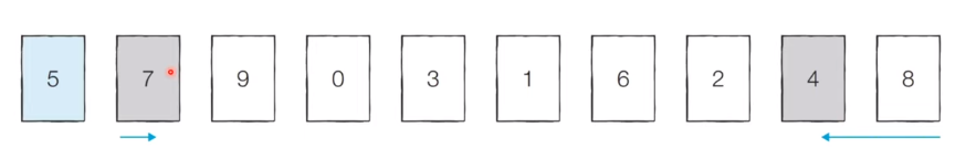
[Step 1]
The current pivot value is 5. Since data larger than 5 is selected from the left, 9 is selected, and since data smaller than 5 is selected from the right, 2 is selected. Now, the positions of the two data are changed to each other. 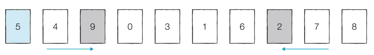
[Step 2]
The current pivot value is 5. Since data larger than 5 is selected from the left, 6 is selected, and since data smaller than 5 is selected from the right, 1 is selected.
However, if the positions are staggered like this, the positions of the pivot and small data are changed. 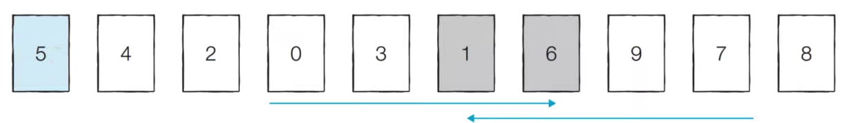
[Divide complete]
Now, the data to the left of 5 are all less than 5, and the data to the right are all greater than 5. This operation of dividing the data bundle based on the pivot is called divide. 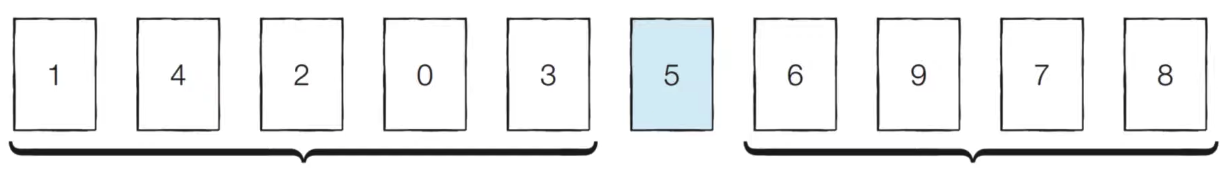
[Left Data Bundle Sort]
Quick sort is performed on the data on the left in the same way. 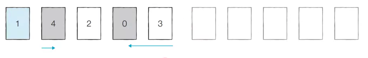
Performed recursively. Every time you do quicksort, the sorting range gets narrower.
[Right Data Bundle Sort]
Quick sort is performed on the data on the right in the same way. 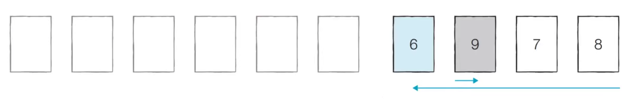
If this process is repeated, sorting is performed on all data.
Why Quick Sort is Fast?
In the ideal case, if the division occurs by half, \(O(NlogN)\) can be expected for the total number of operations. \(Width \times height = N \times logN = NlogN\)
4.2 Quick Sort Implementation
Implementation in a usual way
# title: 'QuickSort1.py'
array = [5, 7, 9, 0, 3, 1, 6, 2, 4, 8]

def quick_sort(array, start, end)
    if start >= end: #end if 1 element
        return
    pivot = start # (otherwise) pivot is the first element
    left = start + 1 #set left
    right = end #set right
    while( left <= right ): #Repeat until crossed
        # iterate until we find data larger than the pivot
        while{ left <= end and array[left] <= array[pivot] ):
            left += 1
        # iterate until we find data smaller than the pivot
        while( right > start and array[right] >= array[pivot] ):
            right += 1
        if( left > right ): #if it crossed
           array[right], array[pivot] = array[pivot], array[right] #Swap the pivot with small data
        else: #if not crossed
            array[left], array[right] = array[right], array[left] # Swap small and large data

    # Perform sorting on the left part and the right part after division
    quick_sort(array, start, right -1 )
    quick_sort(array, right +1, end )

quick_sort(array, 0, len(array) -1 )
print(array)

# output
# [0, 1, 2, 3, 4, 5, 6, 7, 8 ,9]
Implementation in a way that takes advantage of Python’s strengths
# title: 'QuickSort2.py'
array = [5, 7, 9, 0, 3, 1, 6, 2, 4, 8]

def quick_sort(array):
    # quit if list contains no more than one element
    if len( array ) <= 1:
        return array
    pivot = array[0] #The pivot is the first element
    tail = array[1:] #List without pivot (make a list from the 2nd element to the last element)

    left_side = [x for x in tail if x <= pivot] # (if less than pivot value) the divided left part
    right_side = [x for x in tail if x > pivot] # (if greater than pivot value) divided right part

    # After dividing, sort the left and right parts, respectively, and return the entire list
    return quick_sort(left_side) + [pivot] + quick_sort(right_side)

print(quick_sort(array))

# output
# [0, 1, 2, 3, 4, 5, 6, 7, 8 ,9]
Receive the callback function as the second argument, and Sort based on the return value of that function
// title: 'QuickSort3.js'
function quickSort(arr, transform = (item) => item) {
  if (arr.length <= 1) return arr;

  const pivot = arr[0];
  const left = [];
  const right = [];

  for (let i = 1; i < arr.length; i++) {
    if (transform(arr[i]) < transform(pivot)) left.push(arr[i]);
    else right.push(arr[i]);
  }

  const lSorted = quickSort(left, transform);
  const rSorted = quickSort(right, transform);
  return [...lSorted, pivot, ...rSorted];
}
4.3 Time complexity of Quick Sort
Quicksort has a time complexity of \(\underline{O(NlogN)}\) in case of average.
However, it has a time complexity of \(\underline{O(N^2)}\) in the worst case.
What happens if you perform quicksort on an already sorted array when the first element is pivoted? 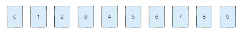
- Segmentation in which only the right data remains is continued.
- The number of divisions is N. (A linear search must be performed every time.)
- Time complexity : \(N \times N => O(N^2)\)
The programming default library is set to implement \(NlogN\) even in the worst case.
4.4 Quick Sort Applications
- the programming language is good for recursion
- time complexity matters
- space complexity matters
5. Counting Sort
5.1 What is Counting Sort?
It is a very fast sorting algorithm that can only be used when certain conditions are met.
Counting sort can be used when the size range of data is limited and can be expressed in integer form.
When the number of data is N and the maximum value among data (positive numbers) is K, the execution time \(\underline{O(N + K)}\) is guaranteed even in the worst case.
[Step 0]
Create a list to contain all the ranges from the smallest data to the largest data.
Data to sort by: 7 5 9 0 3 1 6 2 9 1 4 8 0 5 2 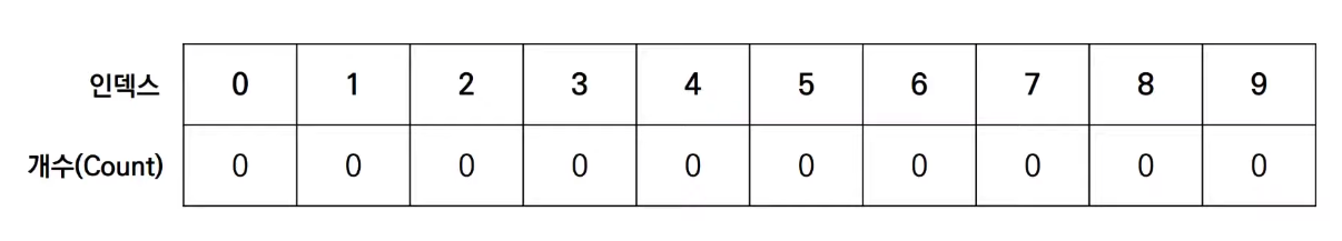
Count the number of times each data appeared in total.
[Step 1]
Check the data one by one and increase the data of the same index as the data value by one.
Data to sort by: 7 5 9 0 3 1 6 2 9 1 4 8 0 5 2 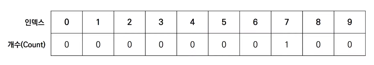
[Step 2]
Check the data one by one and increase the data of the same index as the data value by one.
Data to sort by: 7 5 9 0 3 1 6 2 9 1 4 8 0 5 2 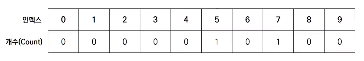
[Step 15]
As a result, the number of times each data appears is recorded in the final list.
Data to sort by: 7 5 9 0 3 1 6 2 9 1 4 8 0 5 2 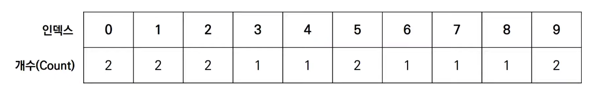
When checking the result, the index is printed by repeating the value one by one from the first data in the list. 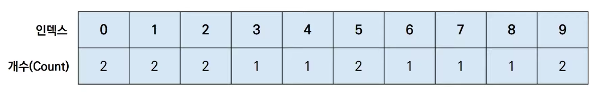
Output Result: 0 0 1 1 2 2 3 4 5 5 6 7 8 9 9
Although the space complexity is relatively high, it operates faster if the conditions are satisfied.
5.2 Counting Sort Implementation
# title: 'CountingSort.py'
# Assume all elements are greater than or equal to 0
array = [7, 5, 9, 0, 3, 1, 6, 2, 9, 1, 4, 8, 0, 5, 2]
#declare a list containing all ranges (all values are initialized to 0)
count = [0] * (max( array ) + 1) # Create a count array with a size of 10 from 0 to 9.
for i in range(len( array )): #Check the number of data (N)
count[array[ i ]] += 1 #Increase the index value corresponding to each data (record how many times it appears)
for i in range(len( count )): #Check the sort information recorded in the list (check each index)
for j in range(count[ i ]): # The number of executions of the inner loop is N.
print(i, end=' ') # Print the index as many times as the number of occurrences separated by spaces
# output
# 0 0 1 1 2 2 3 4 5 5 6 7 8 9 9
5.3 Time complexity of Counting Sort
Both the time and space complexity of Counting sort are \(\underline{O(N + K)}\).
(N: the number to be sorted) (K: the largest value among elements)
Counting sorting can sometimes lead to serious inefficiencies.
- Consider a case where there are only two data, 0 and 999,999. (You must create an array containing 1 million elements.)
Counting sorting can be effectively used when multiple data with the same value appear.
- In the case of grades, there may be several students who scored 100 points, so sorting the counting sort is effective.
5.4 Counting Sort Applications
- there are smaller integers with multiple counts.
- linear complexity is the need.
6. Radix Sort
6.1 What is Radix Sort?
Radix sort is a sorting algorithm that sorts the elements by first grouping the individual digits of the same place value. Then, sort the elements according to their increasing/decreasing order.
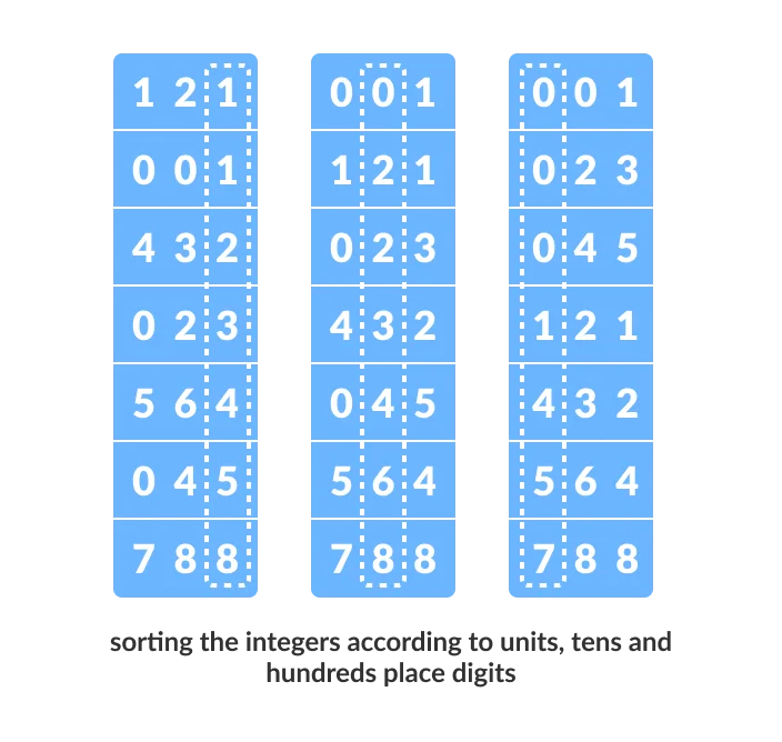
Suppose, we have an array of 8 elements. First, we will sort elements based on the value of the unit place. Then, we will sort elements based on the value of the tenth place. This process goes on until the last significant place.
Let the initial array be [121, 432, 564, 23, 1, 45, 788]. It is sorted according to radix sort as shown in the figure below.
[Step 0]
Find the largest element in the array, i.e. max. Let X be the number of digits in max. X is calculated because we have to go through all the significant places of all elements.
In this array [121, 432, 564, 23, 1, 45, 788], we have the largest number 788. It has 3 digits. Therefore, the loop should go up to hundreds place (3 times).
[Step 1]
Now, go through each significant place one by one.
Use any stable sorting technique to sort the digits at each significant place. We have used counting sort for this.
Sort the elements based on the unit place digits (X=0). 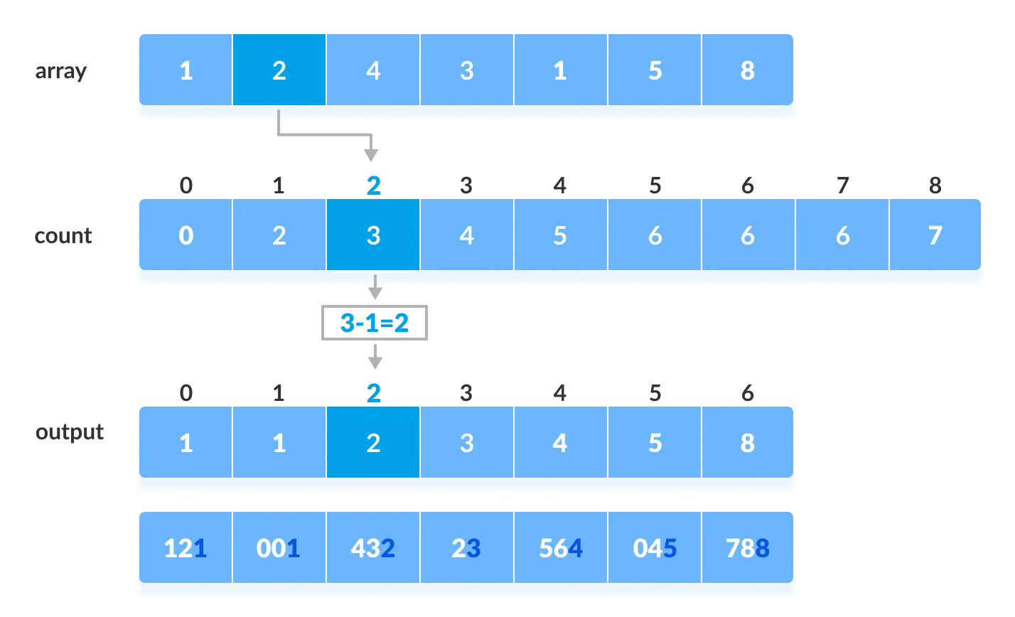
[Step 2]
Now, sort the elements based on digits at tens place. 
[Step 3]
Finally, sort the elements based on the digits at hundreds place. 
6.2 Radix Sort Implementation
# title: 'RadixSort.py'
# Using counting sort to sort the elements in the basis of significant places
def countingSort(array, radix):
    size = len(array)
    output = [0] * size
    count = [0] * 10

    # Calculate count of elements
    for i in range(0, size):
        index = array[i] // radix
        count[index % 10] += 1

    # Calculate cumulative count
    for i in range(1, 10):
        count[i] += count[i - 1]

    # Place the elements in sorted order
    i = size - 1
    while i >= 0:
        index = array[i] // radix
        output[count[index % 10] - 1] = array[i]
        count[index % 10] -= 1
        i -= 1

    for i in range(0, size):
        array[i] = output[i]


# Main function to implement radix sort
def radixSort(array):
    # Get maximum element
    max_element = max(array)

    # Apply counting sort to sort elements based on place value.
    place = 1
    while max_element // place > 0:
        countingSort(array, place)
        place *= 10

data = [121, 432, 564, 23, 1, 45, 788]
radixSort(data)
print(data)
If we need to radix sort all integers (including negative numbers).
- Convert negative numbers to positive numbers while putting them in the left.
- Put positive numbers in right.
- Reverse left and multiply by -1. Then, concat right to sort.
6.3 Time complexity of Radix Sort
| Time Complexity | Space Complexity | Stability | ||
|---|---|---|---|---|
| Best | Worst | Average | \(O(max)\) | Yes |
| \(O(N+K)\) | \(O(N+K)\) | \(O(N+K)\) |
Since radix sort is a non-comparative algorithm, it has advantages over comparative sorting algorithms.
For the radix sort that uses counting sort as an intermediate stable sort, the time complexity is \(O(d(N+K))\).
Here, d is the number cycle and \(O(N+K)\) is the time complexity of counting sort.
Thus, radix sort has linear time complexity which is better than \(O(NlogN)\) of comparative sorting algorithms.
If we take very large digit numbers or the number of other bases like 32-bit and 64-bit numbers then it can perform in linear time however the intermediate sort takes large space.
This makes radix sort space inefficient. This is the reason why this sort is not used in software libraries.
6.4 Radix Sort Applications
- DC3 algorithm (Kärkkäinen-Sanders-Burkhardt) while making a suffix array.
- places where there are numbers in large ranges.
7. Merge Sort
7.1 What is Merge Sort?
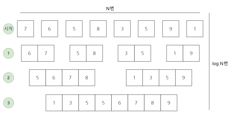
Merge sort divides one large problem into two smaller problems, computes each, and then merges them. That said, the basic idea is to divide it exactly in half once and sort it later.
Unlike quicksort, merge sort has no pivot value and always divides in half. This feature makes the step size logN.
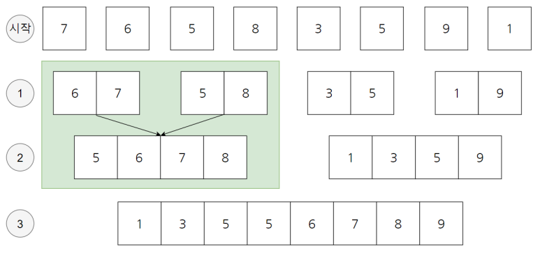
Let’s look at the picture above. All of the 7 6 5 8 3 5 9 1s start out as individual arrays of size 1. Now, in the first step 1, each array is of size 2. It’s a combination of two things that used to be one size. If you look, you can see that in the first step 1 is divided by 6 7 / 5 8 / 3 5 / 1 9. Then the second step is to combine the ones of size 2 by two to create an array of size 4.
In other words, the sort is performed at the moment of merging. The merging step only takes 3 steps. The sum is 2^3 = 8 in the sense that the number doubles, so only 3 steps are needed.
7.2 Merge Sort Implementation
# title: 'MergeSort1.py'
def mergeSort(arr):
    if len(arr) > 1:
        # Finding the mid of the array
        mid = len(arr)//2
        # Dividing the array elements
        L = arr[:mid]
        # into 2 halves
        R = arr[mid:]
        # Sorting the first half
        mergeSort(L)
        # Sorting the second half
        mergeSort(R)
        i = j = k = 0

        # Copy data to temp arrays L[] and R[]
        while i < len(L) and j < len(R):
            if L[i] < R[j]:
                arr[k] = L[i]
                i += 1
            else:
                arr[k] = R[j]
                j += 1
            k += 1

        # Checking if any element was left
        while i < len(L):
            arr[k] = L[i]
            i += 1
            k += 1

        while j < len(R):
            arr[k] = R[j]
            j += 1
            k += 1

# Code to print the list
# def printList(arr):
#     for i in range(len(arr)):
#         print(arr[i], end=" ")
#     print()

# Driver Code
# if __name__ == '__main__':
#     arr = [12, 11, 13, 5, 6, 7]
#     print("Given array is", end="\n")
#     printList(arr)
#     mergeSort(arr)
#     print("Sorted array is: ", end="\n")
#     printList(arr)
Or this coding is also neat.
// title: 'MergeSort2.js'
function mergeSort(array) {
    if(array.length <= 1) {
        return array
    }
    const middle = Math.floor(array.length / 2);
    const left = array.slice(0, middle);
    const right = array.slice(middle);

    return merge(mergeSort(left), mergeSort(right))
}

function merge(left, right) {
    const array = [];

    while (left.length && right.length) {
        if(left[0]< right[0]) {
            array.push(left.shift());
        } else {
            array.push(right.shift());
        }
    }
    return array.concat(left.slice()).concat(right.slice());
}

// Test Code
// (function test() {
//     const testArray1 = [4, 5, 2, 1, 3, 8]
//     const testArray2 = [5, 5, 6, 100, 3, 5, 2, 1, 5, 7, 8888, 4]
//     const testArray3 = [2, 1]

//     console.log(mergeSortTopDown(testArray1))
//     console.log(mergeSortTopDown(testArray2))
//     console.log(mergeSortTopDown(testArray3))
// })()
One thing to keep in mind when implementing merge sort is that the array used for sorting must be declared as a ‘global variable’. If you declare an array inside a function, the waste of memory resources can become very large in that you have to declare the array every time.
As such, merge sort has the problem of inefficient memory utilization in that additional array space to hold existing data is required. (Heap sort solves the memory inefficiency problem.)
Merge sort is usually slower than quicksort, but is a very efficient algorithm in that it is guaranteed to be exactly \(O(N \times logN)\) under any circumstances.
7.3 Time complexity of Merge Sort
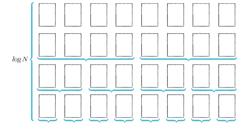
The size of the step is kept as logN when the number of data is N. Also, the execution time required for sorting itself is N. This is because you only need to calculate the number of data. As a result, the total time complexity is \(O(N \times logN)\).
Why is the execution time required for sorting only N? Here’s why it only takes N to sort the subsets.
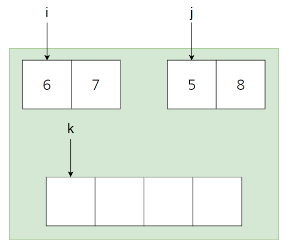
The initial state is as above. In the left set, i points to the first element, and in the second set, j points to the second element. And the array to be sorted is empty. The reason the sort takes only N is the same reason as insertion sort. This is because it assumes that 'the subset is already sorted'. This is because the time complexity of O(N) is sufficient to combine two things that are already sorted.
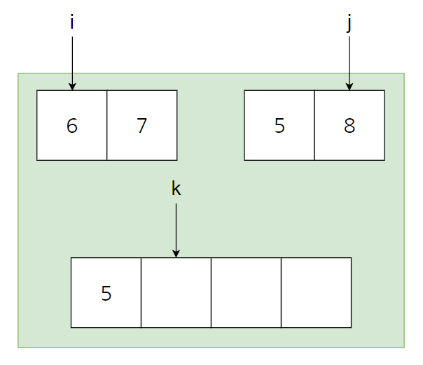
The first process is to compare i and j as above, put a smaller number in the position of k, and add the processed index by one. As a result, you can see that k and j have moved to the right by one space as shown above.
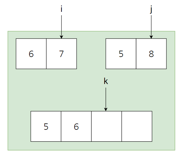
Similarly, comparing i = 6 and j = 8, 6 is smaller, so it is inserted at the k position and i and k are added by 1 each. The result is as above. If you iterate like this, you only need to process exactly N times.
That is, as above, the width is N times and the height is log N times, which guarantees a time complexity of \(\underline{O(N \times logN)}\).
7.4 Merge Sort Applications
- Inversion count problem
- External sorting
- E-commerce applications
8. Heap Sort
8.1 What is Heap Sort?
Heap Sort is a popular and efficient sorting algorithm in computer programming. To write the heap sort algorithm requires two types of data structures - arrays and trees.
Heap sort works by visualizing the elements of the array as a special kind of complete binary tree called a Heap.
Relationship between Array Indexes and Tree Elements
A complete binary tree has an interesting property that we can use to find the children and parents of any node.
If the index of any element in the array is i, the element in the index 2i+1 will become the left child and element in 2i+2 index will become the right child. Also, the parent of any element at index i is given by the lower bound of (i-1)/2.
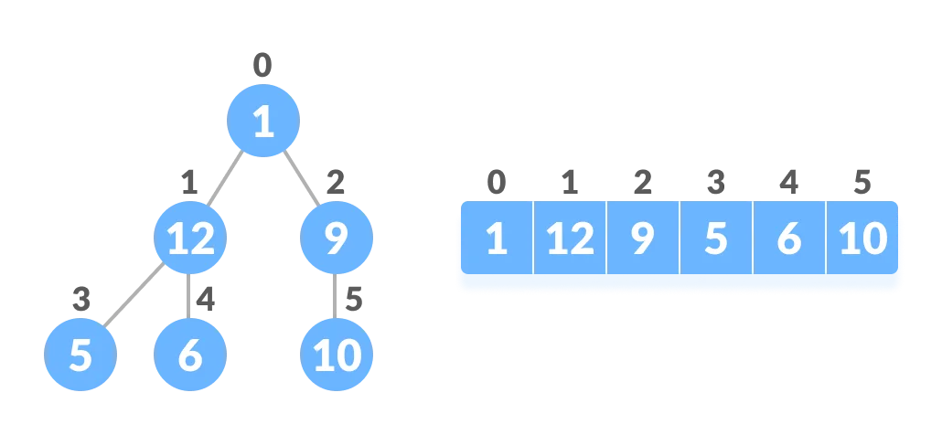
Relationship between array and heap indices
Let’s test it out,
Left child of 1 (index 0)
= element in (2*0+1) index
= element in 1 index
= 12

Right child of 1
= element in (2*0+2) index
= element in 2 index
= 9

Similarly,
Left child of 12 (index 1)
= element in (2*1+1) index
= element in 3 index
= 5

Right child of 12
= element in (2*1+2) index
= element in 4 index
= 6
Let us also confirm that the rules hold for finding parent of any node.
Parent of 9 (position 2)
= (2-1)/2
= ½
= 0.5
~ 0 index
= 1

Parent of 12 (position 1)
= (1-1)/2
= 0 index
= 1
Understanding this mapping of array indexes to tree positions is critical to understanding how the Heap Data Structure works and how it is used to implement Heap Sort.
Working of Heap Sort
[Step 0]
Since the tree satisfies Max-Heap property, then the largest item is stored at the root node.
[Step 1] Swap
Remove the root element and put at the end of the array (nth position) Put the last item of the tree (heap) at the vacant place.
[Step 2] Remove
Reduce the size of the heap by 1.
[Step 3] Heapify
Heapify the root element again so that we have the highest element at root.
[Step 4]
The process is repeated until all the items of the list are sorted.
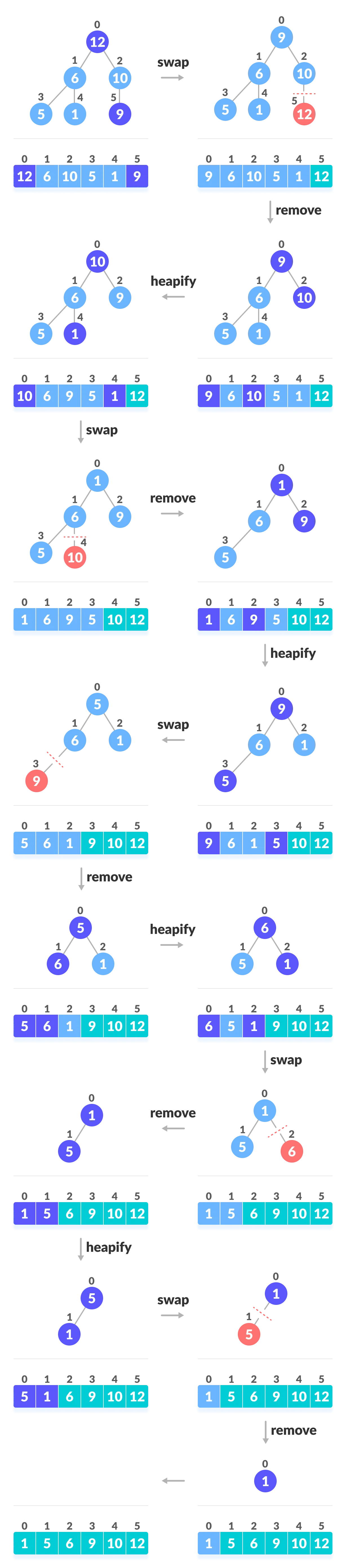
Swap, Remove, and Heapify!
8.2 Heap Sort Implementation
# title: 'HeapSort.py'
def heapify(arr, n, i):
    # Find largest among root and children
    largest = i
    l = 2 * i + 1
    r = 2 * i + 2

    if l < n and arr[i] < arr[l]:
        largest = l

    if r < n and arr[largest] < arr[r]:
        largest = r

    # If root is not largest, swap with largest and continue heapifying
    if largest != i:
        arr[i], arr[largest] = arr[largest], arr[i]
        heapify(arr, n, largest)


def heapSort(arr):
    n = len(arr)

    # Build max heap
    for i in range(n//2, -1, -1):
        heapify(arr, n, i)

    for i in range(n-1, 0, -1):
        # Swap
        arr[i], arr[0] = arr[0], arr[i]

        # Heapify root element
        heapify(arr, i, 0)


arr = [1, 12, 9, 5, 6, 10]
heapSort(arr)
n = len(arr)
print("Sorted array is")
for i in range(n):
    print("%d " % arr[i], end='')
8.3 Time complexity of Heap Sort
| Time Complexity | Space Complexity | Stability | ||
|---|---|---|---|---|
| Best | Worst | Average | \(O(1)\) | No |
| \(O(NlogN)\) | \(O(NlogN)\) | \(O(NlogN)\) |
The height of a complete binary tree containing N elements is log N
As we have seen earlier, to fully heapify an element whose subtrees are already max-heaps, we need to keep comparing the element with its left and right children and pushing it downwards until it reaches a point where both its children are smaller than it.
In the worst case scenario, we will need to move an element from the root to the leaf node making a multiple of \(log(N)\) comparisons and swaps.
During the build_max_heap stage, we do that for N/2 elements so the worst case complexity of the build_heap step is N/2*log N ~ Nlog N.
During the sorting step, we exchange the root element with the last element and heapify the root element. For each element, this again takes log n worst time because we might have to bring the element all the way from the root to the leaf. Since we repeat this n times, the heap_sort step is also Nlog N.
Also since the build_max_heap and heap_sort steps are executed one after another, the algorithmic complexity is not multiplied and it remains in the order of Nlog N.
8.4 Heap Sort Applications
Systems concerned with security and embedded systems such as Linux Kernel use Heap Sort because of the \(O(NlogN)\) upper bound on Heapsort’s running time and constant\(O(1)\) upper bound on its auxiliary storage.
Although Heap Sort has \(O(NlogN)\) time complexity even for the worst case, it doesn’t have more applications ( compared to other sorting algorithms like Quick Sort, Merge Sort ). However, its underlying data structure, heap, can be efficiently used if we want to extract the smallest (or largest) from the list of items without the overhead of keeping the remaining items in the sorted order. For e.g Priority Queues.
9. Sort Algorithm Comparison
| Sort Algorithms | Average Time Complexity | Space Complexity | Feature |
|---|---|---|---|
| Bubble Sort | \(O(N^2)\) | \(O(1)\) | The code is short and simple |
| Selection Sort | \(O(N^2)\) | \(O(N)\) | The idea is very simple. |
| Insertion Sort | \(O(N^2)\) | \(O(N)\) | It is fastest when the data is almost sorted. |
| Quick Sort | \(O(NlogN)\) | \(O(N)\) | In most cases, it is the most useful, and it is fast enough |
| Counting Sort | \(O(N+K)\) | \(O(N)\) | It can be used only when the size of the data is limited, but it works very quickly. |
| Radix Sort | \(O(N+K)\) | \(O(max)\) | It commonly applied to collections of binary strings and integers. |
| Merge Sort | \(O(NlogN)\) | \(O(N)\) | Memory usage is inefficient. |
| Heap Sort | \(O(NlogN)\) | \(O(1)\) | Usually slower than quicksort. |
For reference, the standard sort library supported by most programming languages is designed to guarantee \(O(NlogN)\) even in the worst case.
10. Sort Example Problem
10.1 Problem : Swapping elements in two arrays
I have two arrays A and B. Both arrays consist of N elements, and the elements of the array are all natural numbers.
A maximum of K replacement operations can be performed. A replacement operation means selecting one element from array A and one element from array B and swapping the two elements.
The end goal is to maximize the sum of all elements of array A. Given N, K, and information about arrays A and B, write a program that prints the maximum value of the sum of all elements of array A that can be made by performing at most K replacement operations.
For example, say N = 5, K = 3, and the arrays A and B are as follows.
- Array A = [1, 2, 5, 4, 3]
- Array B = [5, 5, ,6, ,6, 5]
In this case, three operations can be performed as follows.
- Operation 1) Swap element 1 of array A and element 6 of array B
- Operation 2) Swap element 2 of array A and element 6 of array B
- Operation 3) Swap element 3 of array A and element 5 of array B
After the three operations, the states of array A and array B are configured as follows.
- Array A = [6, 6, 5, 4, 5]
- Array B = [3, 5, 1, 2, 5]
At this time, the sum of all elements of array A is 26, and the sum cannot be made larger than this.
Input conditions
In the first line, N and K are entered, separated by spaces. (1 <= N <= 100,000, 0 <=K <= N)
In the second line, the elements of array A are entered separated by spaces. All elements are natural numbers less than 10,000,000.
In the third line, the elements of array B are entered, separated by spaces. All elements are natural numbers less than 10,000,000.
Output conditions
Outputs the maximum value of the sum of all elements of the array A that can be created by performing the maximum K replacement operations.
| Input Example | Output Example |
| 5 3 | 26 |
| 1 2 5 4 3 | |
| 5 5 6 6 5 |
10.2 Solution : Swapping elements in two arrays
The key idea: each time pick the smallest element from array A and replace it with the largest element from array B.
First, given arrays A and B, sort in ascending order on A and sort in descending order on B.
Afterwards, the elements of the two arrays are checked sequentially from the first index, and replacement is performed only when the element of A is smaller than the element of B.
In this problem, up to 100,000 elements in both arrays can be entered, so a sorting algorithm that guarantees \(O(NlogN)\) in the worst case should be used.
# title: 'SwappingElementsInTwoArrays.py'
n, k = map(int, input(). split()) # Get N and K as input
a = list( map( int, input(). split())) # get all elements of array A
b = list( map( int, input(). split())) # get all elements of array B as input

a. sort() # sort array A in ascending order
b. sort( reverse= True ) # sort B in descending order

#Check the first index and compare the elements of two arrays up to K times
for i in range(k):
    #If the element of A is smaller than the element of B
    if a[i] < b[i]
        # replace two elements
        a[i], b[i] = b[i], a[i]
    else: #Escape the loop when an element in A is greater than or equal to an element in B
        break

print(sum(a)) # print the sum of all elements in array A
https://stackabuse.com/
https://www.freecodecamp.org/
https://www.programiz.com/
https://www.geeksforgeeks.org/
https://blog.naver.com/PostList.naver?blogId=ndb796
이것이 코딩테스트다,2020,나동빈,한빛미디어